Chapter 1

Introduction

The purpose of this thesis is to provide implementation details for two filtering algorithms, called edge-finding and max energy, for the scheduling of cumulative resources in constraint-based scheduling. This chapter provides background for these concepts. Section 1.1 introduces the concept of constraint programming. Section 1.2 defines the Cumulative Scheduling Problem, the problem that the edge-finding filtering algorithm will be used to solve. Section 1.3 explains the organization of the remainder of the thesis.

1.1 Constraint Programming

Constraint satisfaction, in its basic form, involves finding a value for each one of a set of problem variables where constraints specify that some subsets of values cannot be used together.

Constraint programming is a declarative programming method for modeling combinatorial optimization problems in terms of constraints. This is a fairly dense statement, so let us address the concepts one at a time.

Declarative programming is a style of programming distinguished from the traditional procedural style. In procedural programming, a problem is solved through the execution of a series of instructions. In contrast, in the declarative style the programmer states the logic of the problem in some form; the procedure of solving the problem so defined is determined by the computer.

In an optimization problem , the goal is to find the best configuration, commonly defined as the maximum or minimum value yielded by a set of functions over several variables; such a problem is combinatorial when there exists only a finite set of possible solutions [25]. The problems generally have concise representations, such as a graph or set of equations, but the number of possible solutions is too large to simply compare them all. While some combinatorial optimization problems are / wereare polynomial, a large class of interesting problems is NP-Complete1,[/annotax] where the number of possible solutions grows exponentially with the problem size [29]. NP-Complete problems are intractable, but often it is possible to find an interesting subproblem that is tractable, or to use a polynomial approximation to find a solution that is at least close to the optimum [19].

Constraints work by reducing the domain of the values that a variable may take in a solution. For example, say the domains of variables X and Y are defined as:

X ∈ {2, 3, 4, 6}
Y ∈ {1, 2, 4, 5}

The constraint X < Y would remove the value 6 from the domain of X, because there is no value in the domain of Y that makes the statement 6 < Y true. Similarlysimilarly , there is no value in the domain of X for which X < 1 or X < 2, so the constraint would remove the values 1 and 2 from the domain of Y. This removal of values is called strengthening the domains of the variables. Constraints never add values to domains. If a constraint removes no values from the domains of any variables in the current state, then that constraint is said to be at fixpoint.

Constraint programming is often defined in terms of the Constraint Satisfaction Problem (CSP), which is: given a set of variables and constraints on those variables, does a solution exist that satisfies all the constraints? For many problems, providing any solution (or demonstrating that no solution exists) is sufficient; for other problems a listing of all solutions is required. Clearly this type of satisfaction problem is less strict than the general combinatorial optimization problem discussed above; however , the CSP can be easily modified to maximize or minimize an objective function, in what is called a Constrained Optimization Problem [3]. The CSP is sufficient for the purposes of this thesis, however.

1.1.1 Example: Sudoku

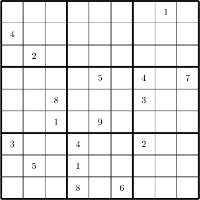
Figure 1.1. A sudoku puzzle with 17 initial values, and exactly 1 solution [28]. The solution is provided in Appendix B.

Sudoku is a popular combinatorial number puzzle, consisting of a 9×9 grid that is further subdivided into 9 non-overlapping 3×3 regions. In a solution , each of the 81 squares in the grid must hold a number between 1 and 9, inclusive; furthermore , solutions satisfy the following conditions:

1. every number in a horizontal row must be different;
2. every number in a vertical column must be different; and
3. every number in a 3×3 region must be different.

In the initial state, several squares have values specified; these values are referred to as hints. The puzzle is solved by finding consistent values for all 81 squares.

These relatively simple rules yield a puzzle that cannot reasonably be solved through simple trial and error. There are 9E81, or slightly fewer than 2×10E77, possible ways to fill out the 9×9 grid, of which approximately 6.67×10E21 are grids that satisfy all three rules [16]. And yet , by fixing the initial values of as few as 17 squares, it is possible to create a puzzle with only one solution [28]. Other grid sizes are possible–we can imagine a hexadecimal suduko where 16 numbers are arranged on a 16×16 grid divided into 44 regions–and the state space is highly exponential, with nE2(n+1)2 assignments possible for an n-sudoku that has a n²×n² grid. It is thereforetherefore no surprise that[/annotax] generalized sudoku has been shown to be NP-Complete [44].

The game of sudoku is easily encoded as a Constraint Satisfaction Problem, however . Each position in the grid is represented by a decision variable (except for positions that correspond to a hint) with an initial domain of [1..9]. Each rule can be encoded as a collection of simple constraints; every rule specifies that the value in a particular cell cannot be equal to any of the values in a set of 8 other cells, so all three rules can be enforced for a single cell through the use of 20 ≠ constraints (there is an overlap of 2 cells between Rule 3 and each of the other two rules, so there are only 20 inequalities for the 24 cells). Taken all together, and throwing out duplicate inequalities, there are 738 inequalities required to model the game.

This formulation is inefficient for the user, who is forced to specify this large number of constraints; it is also inefficient for the constraint solver. Suppose there are three cells, a, b, and c, that are in the same row, with domains

a, b ∈ {1,2} c ∈ {2,3}  (1.1)

With the constraints specified as pairs of inequalities, there are no values that will be removed from the domain of c–for each value of the current domain of c, there exist values in the domains of a and b that make the constraints a ≠ c and b ≠ c true. Yet c = 2 does not actually participate in any solution, since the only possible assignments for the other two variables are {a = 1, b = 2} and {a = 2, b = 1}, either of which will cause the removal of 2 from the domain of c. The problem is that each constraint only knows about two of the variables, so the solver is unable to make deductions that require knowledge of several variables at once.

By encoding the rules as global constraints, this problem is eliminated. Global constraints apply to arbitrary-size sets of variables. Usually global constraints can be decomposed into several simple constraints; the availability of a global constraint not only simplifies the specification of the CSP, but also helps the solver to work more effectively by clarifying the underlying structure of the problem itself [36].

For sudoku solving , the alldifferent global constraint is useful. The most famous and widely studied of global constraints, alldifferent specifies that each of the variables it applies to must take a different value. A set of 27 alldifferent constraints, one for each row, column and region, is sufficient to define the sudoku problem. Figure 1.2 illustrates the use of sequential alldifferent constraints to determine the value of a variable.

Figure 1.2. Application of the three alldifferent constraints to the circled value, showing how the domain is reduced by each constraint. [Figure not shown]

Such an implementation will also perform better in situations like the one described above, if the algorithm that implements the alldifferent constraint is complete, meaning that the algorithm removes from the domains of its variables every value that does not participate in a solution. Fortunately, such algorithms exist for alldifferent, such as the elegant matching theory based algorithm proposed by Regin [26]. Given the domains in (1.1), a complete alldifferent algorithm will use the fact that either a or b must be equal to 2 to eliminate that value from the domain of c.

To solve the sudoku, the 27 alldifferent constraints are evaluated one at a time, possibly removing values from the domains of some of the variables on each evaluation. As the constraints overlap in terms of the variables they cover, several of the constraints will need to be executed repeatedly: each time a variable’s domain is reduced by one constraint, all the other constraints that cover that same variable will need to be reevaluated.

During evaluation , it is possible that the domain of one of the variables will become empty, meaning that there is no solution to the problem that satisfies all the constraints. Otherwise, the evaluation of constraints continues until all of the constraints are at fixpoint; that is, until none of the constraints is able to remove any further values from the domains of the variables. At this mutual fixpoint, if the domain of every variable has only one value, then that fixpoint represents a solution to the puzzle. Puzzles designed for humans are generally of this type: there is one, and only one, solution, and it can be deduced without guessing any of the values.

For some puzzles, there is a mutual fixpoint in which one or more variables still have multiple values in their domains. Puzzles falling into this category are very challenging for humans, but can still be solved easily by constraint solvers by means of a search algorithm. One variable with a domain containing multiple values is chosen, and the domain is fixed to one of the possible values. Using this value, the constraints are evaluated again, reducing all the domains further, until one of the three end states is reached again. If the end state is a solution, the problem is solved; if it is a failure, the solver goes back to the last variable it made a choice for, and makes a different choice; if the end result still has multiple choices for some variables, another is selected and another guess is made. This process is repeated until either a solution is found, or all possible choices have been eliminated.

1.1.2 Solving Constraints

The central idea of constraint programming is that the user defines the problem as a series of constraints, which are then given to a constraint solver. The solver is responsible for the procedural aspects of solving problems, which may be broadly divided into two categories: inference and search.

Inference

Inference is used to reduce the state space by creating more explicit networks of constraints. The constraints that make up the existing constraint network are combined logically to deduce an equivalent, but tighter, constraint network. The process can be repeated until either an inconsistency is detected or the solutions to the problem are found [13]. Compared to brute-force searching, inference provides better worst-case time complexity, but the space complexity is exponential [14].

Since solving the problem directly through inference is too costly, constraint programming generally uses more restricted forms of inference, reducing the state space only partially. This process is called enforcing local consistency, or constraint propagation [13]. The simplest form of local consistency enforced in propagation is node consistency, which ensures simply that the domain of each variable does not contain values excluded by any one of the constraints. More powerful is arc-consistency, which infers new constraints over each pair of variables (values are removed from the domain of a given variable if there exists another variable that cannot take a matching value to satisfy one of the constraints). Stronger types of consistency, such as hyper-arc consistency, path consistency, or k-consistency are less commonly enforced [3].

During propagation, each of the constraints is applied in turn, strengthening the domains of the variables when possible. One constraint may be applied several times, until it reaches fixpoint; once at fixpoint, the constraint can then be ignored until the domain of any of its variables is strengthened, at which point it will need to be executed again until it finds a new, stronger fixpoint. As the constraints of the problem are likely to overlap in their coverage of the variables, a cyclical process of strengthening generally arises. Each constraint strengthens some domains and then, reaching fixpoint, sleeps; this wakes other constraints affecting the variables of the strengthened domains, which results in further strengthening, possibly waking the first constraint once more. Eventually , the strongest mutual fixpoint for all the propagators is reached, and no further propagation is possible [3].

Search

For non-trivial problems, then, inference alone generally does not solve the problem. Any solutions may be found in the remaining, reduced state space; to find these solutions, a search algorithm is used. Search algorithms are ubiquitous in AI and combinatorial optimization methods, which typically use some variant of a heuristic search strategy.

In discussing search strategies, it is useful to think of the state space as a tree. Each node of the tree represents a partial solution; the edges between nodes represent transformations from one state to another [21]. In terms of constraints , the root node represents the state when all the variables have their initial domains. Each child node represents a removal of one or more values from one or more of the variable domains present in the parent node. Taken together, a set of sibling nodes represent all the possible tightened domains of the parent node. The leaf nodes with one value for each variable represent solutions.

In a heuristic search, a simpler (polynomial) calculation is used to determine a promising next step in the search. This heuristic is essentially making an informed guess based on limited information; this guess limits the search space, but there is no guarantee that the best solution, or for that matter any solution, is present in this reduced search space. As a result , heuristic search can get stuck on local optima or even fail to find a solution [21]. The worst-case performance of heuristic search is equivalent to a brute force enumeration of the state space; however , in practice a search with a good heuristic can be very efficient, although the performance of heuristic methods is often highly dependent on the minute adjustment of search parameters [15]. Neither the lack of a guaranteed solution nor the worst-case performance can be eliminated by developing a better heuristic or search technique, as both problems are inherent to the method [19].

The search algorithms in constraint solving are different from the heuristic search in one important way: by enforcing local consistency, the constraint solver only removes non-solutions form the search space. Depending on the search strategy used, a heuristic might fail to find a solution that was present in the original state space; constraint inference, however , is guaranteed to leave that solution in the reduced state space, so that it must eventually be located in a search [17].

The search algorithm employed in a constraint satisfaction problem is backtracking. Backtracking is the foundational search method in AI, and works as follows: viewing the state space as a tree, backtracking starts at the root and proceeds by selecting a child node; the process is repeated until a leaf node is reached. If the leaf node is a solution, the search terminates; if the leaf node represents an inconsistent state, the search moves back through the visited nodes until it reaches the most recently visited node that has as-yet unvisited children. Selecting one of these children, the search then proceeds as before, continuing until either a solution is found or the state space is exhausted [21].

In constraint programming , backtracking is intertwined with propagation to create an efficient search method. It has already been described how inference is used to reduce the initial state space; viewing the space as a tree, subtrees that demonstrably cannot hold solutions are pruned before the backtracking algorithm selects the next node. By selecting a child node, the search algorithm is further reducing the domain of one of the variables. At this point, propagation is repeated, thus tightening domains again; from the view of the state space tree, some nodes are pruned from the subtree rooted at the current node. If this process results in an inconsistent state (i.e., a variable with an empty domain), the search backtracks to the most recently visited node with unvisited child nodes, restoring the domains of the variables to the state represented by that node, and the search continues from there [17].

1.1.3 Formal Definition

The informal definition of constraint programming given above is fairly broad, and can be applied to many different constraint systems. For a more formal treatment , we will restrict ourselves to one of these systems in particular, and consider only finite domain constraint solvers, in which variables are constrained to values from given, finite sets. These domains can be defined by enumerating each member of the set, or as a bounded interval; enumerated domains allow the constraint solver to tighten the domains more, but are only tractable for small domains [18].

We start by defining the Constraint Satisfaction Problem. This definition, as well as the remainder of this section, is adapted from the presentations in [32, 30].

Definition 1.1 (CSP). A constraint satisfaction problem (CSP) is a triple <X, D, C> where

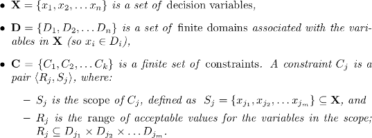
The objective of a CSP is to find a solution: an assignment of values to all the variables that satisfies all the constraints of the problem.

[The remainder of Section 1.1 and Section 1.2 is not shown.]

1.3 Structure of this thesis

The focus of this thesis is on recent work done by Vilím on cumulative scheduling problems. In earlier work 37, 42, 38, Vilím developed versions of several disjunctive scheduling algorithms with complexity O(n log n) using a novel data structure called the Θ-tree. In [39], he uses an extension of this data structure to provide an elegant algorithm for cumulative edge-finding, with a complexity of O(kn log n). In [40], he again uses the Θ-tree to develop an energetic filtering algorithm, which allows for filtering of tasks with variable duration and/or capacity requirements. This thesis presents an implementation of these two algorithms.

Chapter 2 provides a general discussion of edge-finding algorithms, and an overview of the new algorithm proposed by Vilím [39]. Chapter 3 discusses the data structures required by the algorithm in regards to implementation. Finally, several portions of the algorithm that are not discussed in detail in [39] are fleshed out more thoroughly, such as the need for overload checking, an efficient method for α-β-tree cutting, and the symmetry of earliest start time and last completion time adjustment. Chapter 4 presents a discussion of the possibility of parallelizing the edge-finding algorithm. The performance of some different parallel implementations is analyzed. Chapter 5 considers the max energy filtering algorithm proposed by Vilím [40] in detail. Modifications to the Θ-tree structure, required by the algorithm, are reviewed, and a pseudo-code implementation is presented.

1.4 Contributions

The main contributions of this thesis are as follows. Several portions of the edge-finding algorithm in [39], which were either omitted or discussed only in brief in the original paper, are developed more fully here, such as the most appropriate choice of data structure for the Θ-tree, the proper use of the prec to retrieve detected precedences, and several factors which affect loop order in the adjustment phase. Most significantly, a complete algorithm is given for performing the O(log n) cut of the Θ-tree during the update calculation. Several minor improvements to the algorithm are outlined here, such as the elimination of an O(log n) search procedure in the detection phase. Also, some errors in the original paper are identified, including one significant theoretical error, and an incorrect formula provided in one of the algorithms. Additionally , a parallel version of the Θ-tree edge-finder is given here, as well as a combined edge-finding/max energy filter.

 

Footnote

1 A detailed discussion of complexity and intractability is beyond the scope of this work, but a few basic definitions may be helpful for the uninitiated reader. Optimization problems can be divided into two classes, based on how quickly the time required to solve the problem grows as the size of the problem instance grows. Problems for which there exists a solution algorithm that completes in a time that grows in a polynomial fashion with the problem size fall into the set P. Then there is another set of problems, for which there is a polynomial algorithm that can verify the correctness of a solution, but no known algorithm to find a solution in polynomial time; these problems are called NP problems. The hardest of the NP problems, those that are at least as hard as any other problem in NP, form the subset NP-Complete. It is generally supposed that there is no overlap between P and NP-Complete problems (i.e., that NP-Complete problems cannot be solved in polynomial time, instead of having as-yet undiscovered polynomial algorithms), although this conjecture, known as P = NP, remains unproven. There is also a broader class of very hard problems, those that may not even have a polynomial algorithm for verifying solutions; these problems are called NP-Hard. Many rigorous discussions of NP-completeness and intractability are available, primarily [19].