2 Background

Behind the production of forecasts for convection there are many steps and ingredients. Most forecasts are built on numerical atmospheric models that simulate a progression of the present state of the atmosphere. To build such a model it is necessary to have an accurate understanding of the atmospheric physics that explain the processes that are likely to follow. In the simulation stage there is the need for initialization conditions, boundary assumptions and parameterizations. Finally, a very large part of modelling is the numerical methods that step equations of motions forward in time.

In this section, a basic description of the physics behind convection is included. It is followed by an introduction to some key aspects in the modelling of convection. After that, an attempt is made to explain how a forecaster works to produce forecasts of this kind. Finally, a short summary of the various aviation hazards accompanying CB and thunderstorms is added.

2.1 The physics of convection

Thermal atmospheric convection most often occurs during warm summer days. The sun then has the ability to heat the ground so much that the closest air to the ground in the atmosphere gets warmer than the air above. This will make it buoyant and start to ascend in a state of instability. If the air continues to ascend it will eventually reach a level where the water vapour contained in the air will condense into tiny water droplets, forming the first stages of a cloud. Moist convection has then occurred. More often than not, these clouds will only become small tufts known as cumulus or fair-weather-clouds while in certain atmospheric circumstances a few of them might continue to grow vertically because of excessive local updrafts. This may lead to large towering cumulus (TCU ) or even cumulonimbus (CB) where the cloud usually reaches the top of the troposphere and is unable to rise any further. This is called deep convection, as opposed to shallow convection.

Favourable conditions for deep convection are sufficient water vapour in the atmosphere to create and maintain the cloud together with a deep layer of thermodynamic instability and some sort of trigger mechanism causing the air to rise (McIlven, 2010). For thermal convection, the trigger is the sun’s heating of the ground.

For free convection to occur the layer of atmosphere must be unstable, meaning a theoretical air parcel that is displaced from its position must start accelerating in the direction of displacement. The parcel theory assumes an adiabatic process in which the parcel cannot exchange any heat or mass with its surroundings (McIlven, 2010). What determines the atmosphere’s stability is the varying Environmental Lapse Rate (ELR ) and its relation to the dry and moist adiabatic lapse rates (Beychok, 2013). In reality , the atmosphere is only unstable locally and temporarily since it constantly strives to regain neutral conditions.

Conditionally unstable conditions are more common. This is the case where the atmosphere is unstable for a saturated air parcel, but stable for dry air. This is explained by the difference in the dry and wet adiabatic lapse rates. An air parcel at ground level is usually unsaturated, theoretically following the dry adiabatic lapse rate making it stable in these conditions. As a result it takes a certain amount of energy to lift or force the parcel first to the Lifting Condensation Level (LCL), where the water vapour in the parcel condenses, and then to the Level of Free Convection (LFC) where the parcel’s temperature has become warmer than the surrounding air and will continue to rise freely.

The process of lifting the parcel to the LFC is the key to convective initiation which is the first stage in any kind of convective event (Groenemeijer et al., n.d. ). When convection begins, potential energy contained in bubbles of air is released and converted to kinetic energy as the bubbles move upwards. An index named the Convective Available Potential Energy (CAPE) has been created in an attempt to measure this kinetic energy. CAPE is the parcel buoyancy vertically integrated over the levels between which the parcel is positively buoyant. It is given by the formula presented in equation 1.

where θ is the potential temperature of the air parcel, ‾θ is the potential temperature of the environment, z is the height and g is the acceleration of gravity (Stensrud, 2007). The vertical levels LFC and EL are the Level of Free Convection and the Equilibrium Level respectively. EL is the altitude where the parcel is no longer warmer than the surrounding air, and will therefore stop accelerating upwards (Stensrud, 2007).

The  more positive the CAPE, the stronger the possible convection is likely to become. However , even if the values are positive it actually says nothing about if convection will occur or not. Large regions can have a positive CAPE, but it is known that the areas developing convection, such as convective cells, can be considerably smaller (Trier, 2003). The explanation is that of the atmosphere’s tendency to be conditionally unstable in which a trigger mechanism is needed to lift the air up to LFC. This energy barrier is called the Convective Inhibition (CIN). Provided that a positive CAPE is present, the most critical quantity to examine for convective initiation is CIN (Trier, 2003).

CIN works against convective initiation and is measured in energy per unit mass just like CAPE. The higher the CIN the smaller the probability of convection to develop and the more lift is needed to reach free convection. CIN depends in a complicated way on changes in temperature and moisture and is most easily measured by soundings (Trier, 2003). The CIN for an air parcel can be calculated as the buoyancy vertically integrated over the levels between which the parcel is negatively buoyant. The definition is given by equation 2.

where SL is the starting level of the parcel’s ascent (Stensrud, 2007).

An example of a so-called skew-T diagram is shown in figure 1. In these diagrams CAPE and CIN can be found as the areas between the ELR (black right line) and the ascent curve of an air parcel (orange line). The bigger the area for CAPE and the smaller the area for CIN, the more convective activity can be expected.

There are many factors implicating the possibility of forecasting convective initiation. Trier (2003) suggests that these difficulties emerge from the large variety of atmospheric processes influencing the event. Among others, these are turbulent heat and moisture fluxes and horizontal advections of air. Since the heating of the sun depends largely on the surface condition it is also important to be able to map out the earth’s surface in as much detail as possible. Accurate prediction of convective initiation is partly dependent on the availability of accurate atmospheric profiles of temperature and moisture, but also on sufficient knowledge of the physical processes which trigger and develop convection .

Figure 1 – Skew-T diagram showing examples of CAPE and CIN. Of the two black curves, the left one is the atmospheric profile of the dew point (°C), whereas the right one is the ELR (°C). The orange curve is the temperature profile of a theoretic air parcel ascending adiabatically (°C) (Björck 2015a). Reprinted with permission. [Figure omitted]

2.2 Modelling convection

Most forecasts produced today have their origin in the output of one or more numerical weather prediction (NWP) models. They create simulations of the atmosphere and project them forward in time by the use of mathematical equations. These equations are mostly non-linear partial differential equations of a chaotic nature that cannot be solved exactly (Inness & Dorling, 2013). Small errors will intensify rapidly as the simulation steps forward in time (Lynch, 2008). This is the main reason why it is impossible to make exact forecasts and why we can only make relatively detailed forecasts for a few days ahead.

Simulating convective events such as cumulus and cumulonimbus is a particularly complicated process. The horizontal extension of thermals and small cumulus is about 100 m (microscale) while single cumulonimbus are mainly in the small scale region (up to 10 km) but can stretch into the lower span of the mesoscale region (10 to 100 km) (McIlveen, 2010). To be able to explicitly resolve thunderstorm events including its preceding stages, it is therefore necessary to use models that are no larger than at mesoscale to get the sufficient resolution (UCAR, 2002 ). However , because mesoscale models use a higher resolution than conventional synoptic models, they require a large increase in computational resources which results in the realisation that only limited area predictions are practical to produce. Ideally, one might consider microscale models to be the best ones for predicting thermals and isolated convective cells, but the very fine resolution requires such large computational resources that this results in a very small model area, making the forecasts impractical to use.

In grid-point models, which are the most common, the distance between two grid points define the resolution. However , for a weather element to be resolved in the model, it needs to span over five to seven grid points (UCAR, 2002). A thunderstorm cell is normally about 10km wide (Tost, 2009) which if divided by five would require a grid spacing of 2km . Its developing stage as a towering cumulus might be as small as 2km in diameter (EuMetTrain, 2012) which would not be fully resolved unless the grid spacing was around 0.4km, and a small cumulus would require a grid spacing of about 25m (Stensrud, 2007). This is finer than the resolution of any of the models in use in Sweden today, where the finest has a spacing of 2.5km (Ivarsson, 2015). When the event cannot be resolved, the problem must instead be solved with parameterization.

Many models are based on hydrostatic equilibrium in which it is assumed that the horizontal scale is much bigger than the vertical scale and that the weight of the atmosphere directed downwards cancels out the pressure gradient force directed upwards (Innes & Dorling, 2013). This is true for a stable atmosphere, but untrue in the very local occurrences of instability that cause convection (Huang, 2010). Convection entails significant vertical motion and a vertical scale that is about the same size or even larger than the horizontal scale, making a hydrostatic approximation inappropriate when dealing with CB and thunderstorms (UCAR, 2002). However, since convection is so local and acts to restore the stability in the course of a few hours, a hydrostatic approximation is still sufficient for many applications (Huang, 2010).

Models that do not make the assumption of hydrostatic equilibrium are called non-hydrostatic models. They are often high-resolution mesoscale models and usually include a set of equations describing vertical movement that the hydrostatic models do not consider. The main equation states that, in a model grid box, the change in vertical motion with respect to time equals the changes due to advection and local buoyancy minus the non-hydrostatic vertical pressure gradient and the drag from precipitation. This allows the models to forecast changes in atmospheric buoyancy and the potential for convection in more detail (UCAR, 2002).

According to UCAR (2002), concerning high-resolution non-hydrostatic models, “the model forecasts include features such as a system’s abrupt leading-edge gust front and associated temperature change, the thick anvil and its effect on surface temperature as well as the trailing mesohigh and its impact on surface winds”. However , along with this high level of detail also comes a large potential for error as the high-resolution non-hydrostatic models comprise a great sensitivity for small deviations in atmospheric structure. Furthermore , there is the implication of a much higher demand in computational resources because of all the extra equations to be solved as well as a demand for shorter time steps in the numerical solutions. The details thus become false accuracy if the model initialisation, boundary conditions or simulation of the convective initiation is lacking or erroneous.

Jolliffe & Stephenson (2012) describe high-resolution models as giving forecasts where “the realistic spatial structures in the forecast fields provide useful information for users, but getting the forecast exactly right at fine scales is difficult or even impossible due to the chaotic nature of the atmosphere”. The forecasts are therefore often interpreted with some uncertainty, “i.e. ‘about this time, around this place, about this magnitude’, rather than taken at exactly face value” (Jolliffe & Stephenson, 2012).

2.2.1 Parameterization

To overcome the problems of certain events not being resolved by the models, parameterization is used. Different features associated with the event are then replaced with a single estimated value for each model variable in each grid point (Stensrud, 2007). For low resolution models , parameterization is used for both shallow and deep convection, while high resolution models (~ 2.5km) only need to use it for shallow convection.

There are several parameterization “schemes” for processes induced by convection, ranging from convective initiation to deep convection, including the vertical motions trapped in a CB cell and the precipitation produced (UCAR, 2002). The schemes calculate changes in environmental temperature and the specific humidity for each grid box. Some are also coupled with the variables of momentum in the model (Stensrud, 2007).

Different schemes can be characterized and approached in several different ways. For example, there is a significant difference between low-level control schemes and deep-layer control schemes. A low-level control convective scheme approaches convective initiation and development from the removal of CIN by small-scale forced lifting. A deep-layer convective scheme generally uses an approach of reducing the CAPE generated by the large-scale surroundings by applying convection (Stensrud, 2007). To transfer the information derived by the parameterization equations to the grid point model, a set of closure assumptions is applied. These assumptions translate the derived results to effects on the model variables, giving them adjusted values (Stensrud, 2007).

A few of the many available possibilities when using different convective parameterizations are direct prediction of precipitation amount (allowing the precipitation to last beyond that of one simulation time step) more realistic prediction of relative humidity fields and better estimation of cloud distribution and the local radiation budget (Stensrud, 2007).

Drawbacks are large computational as well as economic costs. There will also be delays in the so called spin up process which can result in underestimations of precipitation and cloud amount early on in the prediction sequence. The schemes are also rather sensitive to inaccurate initial conditions and insufficient observations (UCAR, 2002). Additionally , as an effect of the significant complexity of parameterizations and the way different parameterization schemes affect each other, many errors can be created in a forecast that are hard to trace (UCAR, 2002). Because of the many links between the different schemes, simply improving one of them is usually not enough to improve the forecasts (Stensrud, 2007).

An example of a convective parameterization scheme is the Kain-Fritsch scheme (Kain & Fritsch, 1990) which was first presented in 1990 but has been updated many times since. It is a low-level control scheme and uses a CAPE closure. It makes an assumption that only one convective event can occur within one mean grid-box of the model at the same time which suggests sensitivity to grid-spacing (Stensrud, 2007).

Another example is the eddy-diffusivity/mass-flux scheme (EDMF) which handles dry and shallow cumulus convection. It parameterizes small eddies with an eddy-diffusivity approach and thermals with a mass-flux contribution (Soares et al., 2004). This scheme combines turbulent and convective parameterizations resulting in fewer problems caused by interference of different schemes (Teixeira et al., 2012).

2.3 Forecasting methods

In the making of weather forecasts, most forecasting centres use one or more NWP-models. However , this is not the only thing determining the final forecast. Forecasts up to a few hours are made from nowcasting (WMO, n.d.) where the forecasters mainly look at observations and then use their own experience to tell in what way the weather is likely to change (Inness & Dorling, 2013). This is partly because the computers need some time to initialize, and by the time the forecasts are done, there are usually more current observations at hand for the forecaster to analyse.

For forecasts up to twelve hours (very short range forecasts) the main method for a forecaster is still to extrapolate the observations, but some consideration for the NWP-forecasts is taken (SMHI, 2015a). Short range forecasts from 12 to 24 hours have an equally large contribution from the forecaster’s extrapolating skill as from the NWP-forecasts, while 24–48 hour forecasts are made by the forecaster evaluating different model outputs and choosing the right one or making some kind of combination for the final forecast product (SMHI, 2015a).

Ultimately, medium range forecasts (3–10 days) (WMO, n.d.) are usually developed as an ensemble of forecasts with outputs caused by slightly different initiation values (Inness & Dorling, 2013). This provides information about the stability of the model outputs and how reliable they are. From this, probabilistic forecasts can be made (Inness & Dorling, 2013).

Forecasting specific convective weather is complicated by the fact that no model today can resolve shallow convection and only a few are able to resolve deep convection. Also, not all models explicitly categorize the weather as convective but simply give outputs of different fields at different levels and information about rainfall and cloud coverage (Björck, 2015b). A skilled forecaster can recognize convective weather in the outputs of the models, but to get a better understanding they usually examine soundings (from in situ observations, by satellites or simulated) with information about the vertical profiles of temperature and humidity. These are discussed further in section 2.3.1 together with so-called indices.

As far as forecasting specific aviation hazards goes, many products eliminate the risks for turbulence and icing in convective clouds since such risks should always be expected and are thus implied if mention of convective events is made (SMHI, 2015d). For more details, a forecaster can get an indication of the degree of turbulence from looking at values of CAPE which is correlated to the vertical speeds of the convective cloud (Groenemeijer et al., n.d.).

Risk for hail can also be deduced by examining the fields of precipitation and the vertical distribution of temperature and humidity inside potential convective clouds. Some of the important factors to account for are elevation, freezing level, wet bulb zero level and CAPE (Haby, n.d.). Icing conditions are often found in sub-zero degrees within a layer that is unstable, has an inversion on top and inhabits wind shears (Jakobsson, 2015).

2.3.1 Soundings and indices

To get an indication of the probability of events not directly produced as a field in the forecast, indices are often used. They give a one value indication of the probability of a certain event at a certain position. Numerous indices have been developed specifically to warn for convection, thunderstorms and severe weather. Some of them, used in the models evaluated in this study, are listed below. They all in some way consider the stability of the atmosphere by using data from vertical profiles of temperature and humidity. These profiles can come from soundings by radiosondes and satellites or simulated soundings from numerical models (Groenemeijer et al., n.d.).

The soundings can also tell the forecaster what conditions are necessary for convective clouds to develop and how large they might grow. The temperature at the top of a potential convective cloud can tell whether there is risk for precipitation or even thunder. For this, threshold values have been empirically derived (Björck, 2015a). The height of the tropopause can give an indication of the possible strength of a thunderstorm reaching through the entire troposphere. The humidity of the surrounding air is also of significance as entrainment of dry air can hold back the process. Moreover , the wet bulb temperature of a droplet when it has reached the ground can tell whether or not the precipitation has a chance of reaching the ground (Björck, 2015a).

When nowcasting is being done , observational in situ soundings can be used and the information can be extrapolated by the forecaster. However , these soundings have high operational costs and are sparsely used. Simulated soundings, on the other hand, can be put together from the output of most models at every grid point in space for every time step (HIRLAM consortium, 2012, Bouttier, 2009). They enable the forecaster to make the same kind of forecast but with better spatial and temporal resolution and also present soundings that are forecasted themselves. Such forecasted soundings are sensitive to simulation errors, but might be useful for very short range to short range forecasts.

An index that has been used for a long time is the cloud top temperature: the colder the top, the higher the cloud. Traditional rules of thumb that forecasters use say that if the top temperature of a convective cloud has come down to –10°C there will probably be rain, and if it is as low as –30°C, thunder should be expected (Fyrby, 2015). However , this requires that there really is a large vertical distribution of the cloud, which might not be the case. Therefore , another index normally combined with the cloud top temperature is the cloud base level.

The potential energies CAPE and CIN discussed previously can also be used as indices. CAPE can give an indication of the updraft strength of potential convective clouds and CIN can suggest the likelihood of a convective cloud to form at all (Trier, 2003). Even when strong thermals are present, values of CIN over 100 J/kg are typically too large to overcome and convection is very unlikely to develop at all (Groenemeijer et al., n.d.).

For CAPE, values below 300 J/kg usually means no convective potential unless for strong wind shears (Groenemeijer et al., n.d.). Values between 300 and 1000 J/kg imply weak convective potential, 1000 to 2500 J/kg means moderate, and values above 2500 J/kg indicate strong convective potential (Skystef, n.d.). In the environment of severe thunderstorms, it is possible for CAPE values to exceed 6000 J/kg (Stensrud, 2007).

However , even though CAPE represents an air parcel’s theoretical kinetic energy, in reality it is not fit to present the updraft speed of the parcel. This is because of the many assumptions behind the calculations which include neglecting entrainment (i.e. mixing between the parcel and the environmental air), pressure perturbations and the weight of water droplets and ice (Groenemeijer et al., n.d.).

Another index is the KO-index (konvektiv-index), which was designed to account for low and mid-level potential instability (Haklander & Van Delden, 2003). It is calculated as shown in equation 3.

where θi is the equivalent potential temperature of the atmosphere (°C) and i is the pressure level (hPa) (Haklander & Van Delden, 2003). A KO-value of more than 6 indicates no risk of thunderstorms while a value less than 2 says that thunderstorms are likely (EUMeTrain, 2007).

Yet another example is the K-index, which is defined by equation 4 (Haklander & Van Delden, 2003).

where Ti is the temperature (°C), Tdi is the dew point temperature (°C) and i is the pressure level. Values above 20 indicate some potential for thunderstorms, while values above 40 usually always result in thunderstorms (University of Wyoming, n.d.).

Other indices exist that directly address the risk for large hail, severe winds and icing. However, no index gives a straight answer to whether or not there will be convective events or how strong they will be. The real life atmosphere is a lot more complicated than any of the calculations behind the indices. Some might be reasonably good indicators in certain areas but useless in others, often depending on if the area is similar to the one over which the index was constructed (Groenemeijer et al., n.d.). As in all aspects of forecasting, making an estimate from several different indices would probably result in the best possible forecast.

2.4 Forecast verification

An important part of the world of forecasting is verification. Forecasts are meant to be as accurate predictions of the future as possible, but they are far from perfect. As a way of quantifying how skilful or valuable a forecast has been, a variety of verification methods exist, most using numeric verification scores.

Jolliffe & Stephenson (2012) discuss the procedures of forecast verification and suggest that when it comes to meteorological phenomena, many events can be seen as binary, i.e. they either did or did not occur. Examples are rainfall, frost and lightning. For such events, so called yes/no forecasts can be made. If a yes/no forecast predicted an event which did occur, it is regarded as a hit (a). There is also the possibility of a forecast predicting an event that did not occur, which is then regarded as a false alarm (b). If a forecast failed to predict an event that did occur, it is a miss (c). Finally, a forecast can correctly predict the absence of an event, which is then labelled a correct rejection (d) (Jolliffe & Stephenson, 2012). These possible outcomes are often seen in the form of a contingency table (table 1) and are used to calculate many different verification scores. Hits and correct rejections are regarded as positive outcomes and result in a reward to the score, while misses and false alarms give penalty to the score.

Jolliffe and Stephenson (2012) also bring up the implications of “double penalty” which is common among fine scale models. It is said to occur when there is a small position error of a binary event, resulting in the forecast being penalized both for false alarm, i.e. predicting an event where it did not occur, and for failing to predict the event where it actually did occur (missing) (Jolliffe & Stephenson, 2012).

Spatial forecasts, such as those produced by grid-based NWP models, are often treated in alternative ways when it comes to verification. Instead of getting a score from each individual grid point, a method known as neighbourhood verification can be used. The verification is then done for varying neighbourhood sizes, i.e. a varying number of grid boxes included when calculating the score, where the smallest size is one grid box. This is a way of checking for what resolution the forecast is useful.

Neighbourhood verification methods reduce the risk for double penalty, since according to Jolliffe and Stephenson (2012), “neighbourhood methods relax the requirement for an exact match by allowing forecasts located within special neighbourhoods of the observation to be counted as (at least partly) correct”. This being considered, “the neighbourhood verification methodology is perfectly suited for a comparison of the skill of models with different horizontal resolutions” (Weusthoff et al., 2010).

One widely used neighbourhood verification score is the fractions skill score (FSS) (Roberts & Lean, 2008) presented in equation 5. The score rewards forecasts being nearly accurate in space and can be regarded as the probability for an event to occur within a neighbourhood of a given size (Björck, 2010).

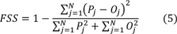
where P is the fraction of forecasts of an event (a+b) and O is the fraction of observed events (a+c) over the grid points of a defined domain. The score averages over a total number or neighbourhoods N and varies between 0 (complete mismatch) and 1 (perfect forecast) (Björck, 2010).

To supplement neighbourhood verification, calculations of frequency bias can be done as shown in equation 6. This is simply a fraction of the forecasted events to the occurred events. It indicates whether the forecast tends to predict the event more or less frequently than it is actually observed (Inness & Dorling, 2013).

Another score is the Gilbert Skill Score (GSS), also known as the Equitable Threat Score (ETS), presented in equation 7. It is an adjustment of a simple score known as the Critical Success Index (CSI) which gives the probability of a hit, “given that the event was either forecast, or observed or both” (Jolliffe & Stephenson, 2012). The adjustments made for the ETS takes into account the probability of forecasts making a hit purely by chance.

where ar = (a + b)(a + c)/n and n = a + b + c + d, i.e. the total number of forecasts (Jolliffe & Stephenson, 2012). The score is best used for events that are pretty rare, since the number of correct rejections is not taken into account.

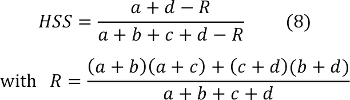
Finally, yet another score that gives credit to correct forecasts that were not merely due to chance is the Heidke Skill Score (HSS) defined in equation 8 (Kunz, 2007).

 

2.5 Aviation hazards in the vicinity of CB and thunderstorms

There is a large variety of phenomena caused by CB and thunderstorms that could be dangerous for an aircraft to be objected to. Perhaps the most prominent danger is the turbulence associated with such weather. Turbulence can cause excessive loads on the aircraft structure, risking structural damage as well as creating a dangerous True Air Speed (TAS) of the aircraft, either making it dangerously high or fatally low. It can also cause the pilot to force the airplane into an unsafe attitude (i.e. a too large or too small angle of attack of the airflow to the wings) in an attempt to maintain a constant altitude. This might lead to stalling where the lifting force of the airplane is lost after which crashing is sometimes unavoidable (Air Ministry Meteorological Office, 1960).

The turbulence is most severe in the core of the thunderstorms where the convective updrafts are at their strongest, but it can extend beyond the cloud as well. Surrounding a TCU or CB there are downdraughts as a result of the circulation of air from the convective cells (Oxford Aviation Academy, 2008). These may cause severe turbulence up to a distance of 30km from a vigorous thunderstorm (Florida International University, 2008). Up- and downdrafts can also be found underneath the cloud, sometimes resulting in a phenomenon known as microburst. This imposes severe wind shear conditions as well as extreme turbulence in an area of 1–5km underneath the cloud (Oxford Aviation Academy, 2008).

The next great hazard is the high probability of “icing” inside the cloud. This means that ice is accumulated on the wings and frame of the aircraft which increases aerodynamic drag, makes the airplane heavier, and disturbs the airflow over the wings. These are all factors capable of highly reducing the amount of lifting force available, again introducing the risk of stalling.

Other hazards are poor visibility in the showers underneath the cloud and large hail, the latter capable of causing structural damage to an aircraft. Getting struck by lightning should be avoided, but it is not as dangerous as generally believed. All aircraft have devices to lead the electricity from lightning strikes back into the atmosphere, and it is very uncommon for the aircraft to be affected at all.

Small airplane pilots usually stay clear of these clouds, partly because of the well-known dangers inside it, but also because most of them follow different operational rules than larger airplane pilots do. These are called Visual Flight Rules (VFR) and essentially state that the pilot needs to be able to ‘see where he ’s going’ which implies not being allowed to fly through clouds or in areas with very limited visibility. Hence , icing and turbulence within the clouds are not direct hazards for small airplane pilots even if they are crucial to pilots who do fly through clouds.