2. Methodology

In this chapter , the pursuit of a measure of human capital will be set in the context of an omitted variable problem. The technical coherency is heavily indebted to the illuminating work of economist Jeffrey M. Wooldridge (2010). However , for a general solution to an omitted variable problem to work on our particular problem of estimating human capital, two assumptions must hold. First, that the characteristics of an individual that are unobservable (at least to the econometrician), but nevertheless fundamentally connected to the concept of human capital, constitute a source of time-invariant variation between individuals’ productive capacities. Second, that this in turn incurs variation in the wages between individuals in proportion to the market value of their unobserved characteristics. Under these assumptions, the problem of estimating the effect of the unobservable characteristics can be equated to the problem of obtaining an estimate of the variation of production capacity between individuals that is left unexplained after observable time-varying factors have been controlled for.

I realize that some of the mathematical expressions and derivations in this chapter might come off as a tad explicit, and maybe even pedantic, in the eyes of the reader. And I would tend to agree with that assessment. Even so, due to the novel nature of the methodological approach to obtain measures of human capital in this paper, I’m afraid I feel it is necessary to harass the reader in this way. But should the reader be endowed with previous experience of estimating unobserved effects via fixed-effect regression, or for some other reason be confident in the validity of my interpretation of the results to come, the reading of section 2.1 in this chapter needn’t be ferociously meticulous.

2.1 The omitted variable problem

The aim of our model is to obtain a measure of human capital at the level of the individual. At our disposal are longitudinal data on a large representative panel of individuals. Since we already established that human capital is manifested in many unobservable characteristics of an individual, a simple OLS regression will result in important variables being omitted. To illustrate the problem thus faced, we specify a linear population model with an unobserved effect Θ entering additively along with the explanatory variables X as follows:

(2.1) E(Y|X, Θ) = Xβ+Θ

Here, X is a N x K matrix of i = 1, 2, …, N observations of the j = 1, 2, …, K explanatory variables, with all the elements in its first column equal to one (enabling an intercept to be estimated). β is a K x 1 vector of parameters of which consistent estimation is of primary interest. Now, if Θ is uncorrelated with X , such that  , omitting Θ will not cause any problems for the estimation of β. Θ will just be another indiscernible influence on Y without any interference on the relationship between X and Y. If Θ on the other hand is correlated with any of the elements in X, say xk , then omitting Θ will result in biased and inconsistent estimation of βk. To see this, we write (2.1) in a simple error form with one explanatory variable in addition to the intercept:

(2.2) y = β0 + β1x1 + Θ + ε

We then derive the OLS estimator of β1 in (2.2):

(2.3)

Now, the first and last term of the third row in (2.3) equals zero since β0 is constant and Cov(ε, x1) = 0 by design. Also, the multiplicand of β1 equals one since a random variable’s covariation with itself is its variance per definition. As is obvious from this exercise, consistent estimation of β by OLS requires that Cov(Θ, x1) = 0.

There are several ways of dealing with the problem of an omitted variable correlating with explanatory variables. One can insert instruments for the elements of X that are correlated with Θ and proceed using an instrumental variable estimator. It is also possible to use a variety of proxy- and indicator variable methods in place of the omitted variable. But what if one isn’t so fortunate so as to have access to such variables? It turns out that with the availability of longitudinal data, new possibilities arise.

The idea for consistently estimating β using variation in longitudinal data is to transform the observations to eliminate the unobserved effect. This is done through the so called fixed effects transformation, where the difference within each cross-section unit between a variable and its mean over time is calculated for each time period. Hence all time-invariant effects are eliminated in the fixed effects model, and consequently become “unobserved”. Bearing in mind that the objective of this study is not to eliminate the influence of the unobserved effects, but to estimate them, I will show in section 2.3 that obtaining unbiased estimates of the unobserved effects from the transformed equations is a trivial task. But for now, suppose we observe the same cross-section units i = 1,2,…,N for t = 1,2,…,T time periods. In our case, the cross-section units correspond to the individuals in the panel. If we also assume that the unobserved effects are time-invariant, we can write the linear unobserved effects model for T time periods as:

(2.4)

Where yit and xit denote observations of cross-section unit i in time period t, and εit denotes the idiosyncratic (i.e. specific to each cross section unit over time) errors. In the next step, we average equation (2.4) over the time periods t = 1,2,…,T to obtain:

(2.5)

Where , , and . Finally, we perform the fixed-effect transformation by subtracting equation (2.5) from (2.4) to attain a fixed effects model:

(2.6)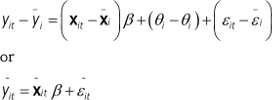

Where by definition , , and . Thus, by time-demeaning equation (2.4) the unobserved effect is eliminated whereby the fixed effects model in equation (2.6) is attained. In the next section, I will discuss the assumptions under which the fixed effect estimator ˆβFE through equation (2.6) will be a consistent estimator of β.

2.2 Assumptions for consistent estimates

Recall the exercise in the previous section where consistent estimation of β by OLS in a linear unobserved effects model required that Cov(Θ, xk) = 0 (see equation (2.3)). This is a very strong assumption about the relationship between the unobserved effect and the explanatory variables. And certainly, in the specific setting of this study such an assumption does not hold. In fact, since we cannot precisely identify the content of the unobserved effect, it would be sensible to allow Θi to be arbitrarily correlated with xit. It will be shown that a fixed effects model achieves this explicitly.

Given the linear unobserved effects model specified in equation (2.4), an assumption of strict exogeneity of the explanatory variables conditional on the unobserved effect can be stated in terms of the idiosyncratic errors as:

(2.7) ,

Implying that, after controlling for the unobserved effect, xit in each time period must be uncorrelated with εit in each time period:

(2.8)

Notice that the assumption in equation (2.7) places no restrictions on E(Θi|xit). This means that the time-invariant unobserved effect Θi can be related to xit in any conceivable way without affecting the consistency of ˆβFE. Thus, Θi is allowed to be arbitrarily correlated with xit, just like we wanted. However , from (2.8) it is clear that assuming zero contemporaneous correlation between xit and εit would be insufficient for consistent estimation. If xis has an effect on yit after xit and Θi has been controlled for when t≠s, assumption (2.7) does not hold.

In addition to the strict exogeneity assumption, we also need to assume that there are no perfect linear relationships among the explanatory variables. This corresponds algebraically to the outer product matrix of the time-demeaned explanatory variable vector ˜xit having full rank. This follows from the fact that the rank of a matrix is equal to its number of linearly independent columns. Hence , the assumption can be stated as:

(2.9)

Now, suppose xit includes a time-invariant explanatory variable, implying that its value never changes for any given cross-section unit. Upon time-demeaning it we would find that its timemean is equal to its value in each time period, rendering the difference between the two equal to zero. Thus the corresponding element in ˜xit would be zero for all time periods, resulting in ˜Xi containing a column of zeroes for all cross-section units. As a result the assumption in equation (2.9) would not hold.

The shattering outcome of including a time-invariant explanatory variable in ˜xit is intuitively appealing for two reasons. First, since fixed effects estimation uses the variation within the cross-section units over time to estimate the population parameters, a variable that does not vary over time for any of the cross-section units cannot be estimated. Second, because Θi is assumed to be time-invariant but allowed to be arbitrarily correlated with xit, it follows that any effects of Θi would be indistinguishable from the effects of a time-invariant explanatory variable in the model. They would both be constant influences.

Under the assumptions of strict exogeneity (2.7), and full rank (2.9), ˆβFE will consistently estimate β. But in order to ensure that ˆβFE is efficient a third assumption about the behaviour of the idiosyncratic errors is needed:

(2.10)

Where σ²ε denotes the variance of εit and IT is an identity matrix. There are two implications of this assumption. First, the variance-covariance matrix  is not allowed to depend on xi or Θi. Second,  should be equal to σ²uIT for all time periods implying that the idiosyncratic errors are serially uncorrelated and exhibit a constant variance for the whole time period.

If the assumptions stated in equations (2.7), (2.9) and (2.10) hold, consistent and efficient estimation of β by fixed effects regression will be achieved. To the extent that they do in our particular setting, I will return to in chapter 4.

2.3 Estimation strategy

The core statistical wage model is:

(2.11)

Where the dependent variable is the logarithm of the wage for individual i at time t, while Θi is a time-invariant person effect, xit a vector of time-varying observable variables, β a vector of their corresponding parameters, and εit the error term. This specification will use the within-variation of each individual to estimate the parameter vector β for the entire sample. Consequently , as long as there is some variation in each element of the time-varying observable variable vector, xit, the influence of those variables will be accounted for among all individuals in the sample.

The idea is then to use the time-invariant person effect captured by Θi, and the experience component of xitβ, to obtain a measure of human capital:

(2.12)

Clearly the different components of h in (2.12) represent different aspects of human capital. To enable a more tangible interpretation of these components, the person effect will be further decomposed into an observed and unobserved part:

(2.13)

Here, zi is a vector of observable time-invariant characteristics and η a vector of their corresponding parameters, while αi constitutes the unobserved dimensions of human capital that is left unaccounted for.

This specification has an immensely important conceptual advantage. Because h in (2.12) contains an unobserved component through the time-invariant person effect Θi, it implies that factors such as cooperative skills, potential, ambition and so on will be included in the measure to the extent that it is compensated through the wage! However , this also connects directly to a potential pitfall of the specification. Since Θi in (2.12) is essentially a “black box” of influences on the wage variable, a successful application of this specification critically depends on the assumption that the sources of variation caught by the parameter are valid components of human capital.

2.4 Obtaining the human capital measure

In this study human capital is defined in equation (2.12) as the sum of the person effect and the experience component of xit. To obtain estimates of the person effects for each crosssection unit, we again consider the linear unobserved effects model for T time periods:

(2.14)

Taking expectations with respect to time on both sides we obtain:

(2.15)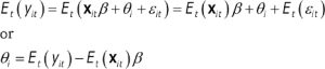

Where E(εit) = 0  by design. Applying the method of moments to (2.15) gives:

(2.16)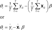 

Where  and . As is clear from equation (2.16), the elements of Θi are intercepts specific to each cross-section unit. Since we can estimate β consistently with ˆβFE, we arrive at an expression from which estimates of the person effect can be obtained:

(2.17) 

Under the assumptions stated in equations (2.7), (2.9) and (2.10), ˆΘi is the best linear unbiased estimator of Θi (Wooldridge, 2010). However , a crucial difference between ˆΘi and ˆβFE is that while ˆβFE is consistent as N → ∞, ˆΘi is not. This follows from the fact that each time a new cross-section unit enters the sample a new element in Θi enters along with it. Thus , increasing the number of cross-section units will not increase the information available for the estimation of Θi implying that although ˆΘi is an unbiased estimator of Θi, it has to rely on asymptotic behavior in the time-domain (T → ∞) for consistency.